Integrating geographic data and the SCS-CN method with LSTM networks for enhanced runoff forecasting in a complex mountain basin
 María José Merizalde1,2*
  Paul Muñoz1
  Gerald Corzo3
  David F. Muñoz4,5 Esteban Samaniego2
  Rolando Célleri1
- 1Departamento de Recursos Hídricos y Ciencias Ambientales, Universidad de Cuenca, Cuenca, Ecuador
- 2Facultad de Ingeniería, Universidad de Cuenca, Cuenca, Ecuador
- 3Hydroinformatics Chair Group, IHE Delft Institute for Water Education, Delft, Netherlands
- 4Department of Civil and Environmental Engineering, Virginia Tech, Blacksburg, VA, United States
- 5Center for Coastal Studies, Virginia Tech, Blacksburg, VA, United States
Introduction: In complex mountain basins, hydrological forecasting poses a formidable challenge due to the intricacies of runoff generation processes and the limitations of available data. This study explores the enhancement of short-term runoff forecasting models through the utilization of long short-term memory (LSTM) networks.
Methods: To achieve this, we employed feature engineering (FE) strategies, focusing on geographic data and the Soil Conservation Service Curve Number (SCS-CN) method. Our investigation was conducted in a 3,390 km2 basin, employing the GSMaP-NRT satellite precipitation product (SPP) to develop forecasting models with lead times of 1, 6, and 11 h. These lead times were selected to address the needs of near-real-time forecasting, flash flood prediction, and basin concentration time assessment, respectively.
Results and discussion: Our findings demonstrate an improvement in the efficiency of LSTM forecasting models across all lead times, as indicated by Nash-Sutcliffe efficiency values of 0.93 (1 h), 0.77 (6 h), and 0.67 (11 h). Notably, these results are on par with studies relying on ground-based precipitation data. This methodology not only showcases the potential for advanced data-driven runoff models but also underscores the importance of incorporating available geographic information into precipitation-ungauged hydrological systems. The insights derived from this study offer valuable tools for hydrologists and researchers seeking to enhance the accuracy of hydrological forecasting in complex mountain basins.
1. Introduction
Hydrological modeling and forecasting are essential for effective water resources management (Wang and Xie, 2018). These tools can be used to develop early warning systems for floods and droughts (Muñoz et al., 2021), or for optimizing hydropower generation through water level forecasting (Hasan and Wyseure, 2018; Falchetta et al., 2020). However, hydrological forecasting remains a challenge in complex hydrological systems. These systems exhibit high spatial variability in geomorphology, topography, and landscape composition, and high temporal variabilities of the main runoff driving forces, such as precipitation and soil moisture. In such complex systems, multiple hydrological processes and runoff generation mechanisms are encountered, making accurate forecasting difficult (Zubieta et al., 2015; Hasan and Wyseure, 2018). The tropical Andes, with their high spatial and temporal variability in climatic conditions and heterogeneity of mountain regions, is an example of a complex basin where accurate hydrological forecasting is crucial for effective water management (Mulligan et al., 2010).
In addition, monitoring hydrometeorological conditions in complex mountain basins, particularly at high elevations, poseses a significant challenge. It is common to find insufficient monitoring networks in such basins, which fail to adequately capture the main drivers of runoff generation (Mulligan et al., 2010; Palomino-Ángel et al., 2019; Llauca et al., 2021). Previous studies have demonstrated that satellite precipitation data can be effectively used for hydrological applications showing promising results. Some of the most-employed satellite precipitation products around the world, are the Integrated Multi-satellitE Retrievals for GPM (IMERG) (Wulf et al., 2016; Palomino-Ángel et al., 2019; Llauca et al., 2021), the Precipitation Estimation from Remotely Sensed Information using Artificial Neural Networks (PERSIANN) (Ma et al., 2018; Palomino-Ángel et al., 2019), and the Global Satellite Mapping of Precipitation (GSMaP) (Huffman et al., 2020). However, while satellite precipitation products can accurately capture spatial-temporal precipitation at large scales, their ability to support reliable hydrological models is limited due to the lack of ground observations in complex systems for validation purposes (Ma et al., 2018; He et al., 2021).
In this context, precipitation-runoff modeling can be addressed using either physical-based or data-driven approaches. Physical-based models use mathematical equations to describe the hydrological process and require detailed system information (Clark et al., 2017). In contrast, data-driven models such as machine learning (ML) models rely on statistical methods to relate input variables with output variable(s) and generally do not provide information about the physical behavior of the system (Solomatine et al., 2008). In recent decades, ML models have become popular among hydrologists due to their advantages, including shorter simulation times, the possibility of computationally inexpensive real-time operation, and less overfitting compared to models based on physical processes (Solomatine and Ostfeld, 2008; Muñoz et al., 2018; Kwon et al., 2020; Adnan et al., 2021; Huang and Lee, 2021; Moreido et al., 2021). The Random Forest (RF) algorithm and the Long Short-Term Memory (LSTM) networks are among the most commonly used ML techniques for hydrological time-series forecasting (Muñoz et al., 2018, 2023; de la Fuente et al., 2019; Campozano et al., 2020; Li et al., 2022; Zhou et al., 2023). Recent studies have shown the superiority of LSTM over RF models for sub-daily runoff forecasting (Zhou et al., 2023). However, regardless of the ML technique used, these models have been criticized for their black box nature, which hinders interpretability and fails to provide a clear roadmap for model enhancement (Shen et al., 2018).
In this sense, the current research trend for achieving model improvement involves the utilization of Feature Engineering (FE) strategies. FE strategies aimed to develop specialized ML forecasting models by strategically integrating process-based hydrological knowledge of the system (Fang et al., 2021; Moreido et al., 2021). FE is a preprocessing step that transforms, creates, and normalizes new inputs into features that can be utilized in ML algorithms. Some FE strategies are for instance the creation of new inputs based on geomorphological factors and hydrometeorological monitoring using Geographic Information System (GIS) techniques (Mahmoud, 2014; Huang and Lee, 2021), and the improvement of precipitation inputs to improve model accuracy (Mahmoud, 2014; Asadi et al., 2019). However, information about the system provided by empirical methods, such as the Soil Conservation Service Curve Number (SCS-CN) (Mishra and Singh, 2003), have been limited and not yet tested in complex basins to add hydrological knowledge to ML models.
The SCS-CN method is an approach used to estimate the amount of runoff from a specific area from precipitation based on the principle that the runoff depends on the characteristics of the soil, antecedent moisture condition, land use/cover (LULC), and topography. For this, empirical equations, along with basin precipitation data, are then used to estimate runoff depth data. This information is critical for understanding the amount of water that will reach nearby streams, rivers, and other water bodies. The applicability of the SCS-CN method to basins with limited ground monitoring stations has made it a popular choice in hydrological modeling since it uses just a single parameter, called curve number (CN), which is derived from established tables of the National Engineering Handbook, section 4 (NEH-4) (Mishra and Singh, 2003). This CN parameter is conditioned by terrain characteristics (LULC, soils, and topography), and represents the infiltration capacity of soils. In this context, GIS plays an important role in developing the SCS-CN method, which allows the handling of the geographical information of soils, LULC maps, and digital elevation model (DEM) to estimate the parameters of the SCS-CN method (Meresa, 2019; Al-Ghobari et al., 2020; Jahan et al., 2021). The SCS-CN method has been assessed globally in multiple basins with varying conditions and characteristics. However, its integration with data-driven models for runoff forecasting has not yet been tested.
In this context, this study aims at developing specialized LSTM runoff forecasting models based on geographic data and the SCS–CN method for a complex basin representative of the Ecuadorean Andes. To achieve this aim, we compare the efficiencies of LSTM specialized and referential (without FE integration) models for lead times of 1, 6, and 11 h, which accounts for near-real-time forecasting, flash floods, and the concentration-time of the basin, respectively.
2. Materials and methods
2.1. Study area
The Jubones basin is located in the southern Andes of Ecuador and has an estimated area of 3,390 km2 when delineated upstream of the Minas-San Francisco (MSF) hydropower plant (see Figure 1). The basin is part of the Andean western slope and ranges in altitude from 771 to 4,100 m above sea level (m.a.s.l.). The Jubones basin has extremely variable climatic conditions with multiple ecosystems and landscapes, influenced by the Andes Mountain range, ocean currents from the Pacific Ocean, and trade winds from the southeast (Hasan and Wyseure, 2018). Consequently, the climate in the basin varies from humid to semi-arid, with annual precipitation regions ranging from 290 to 925 mm (Muñoz et al., 2023).
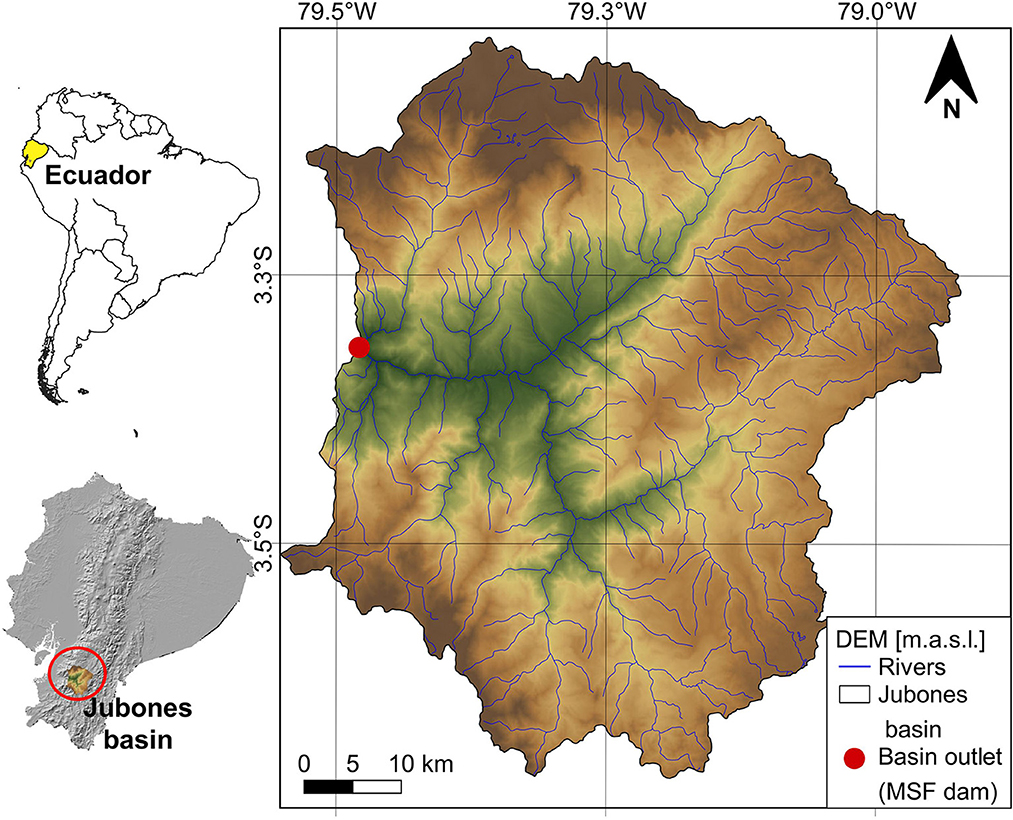
Figure 1. The Jubones basin in southern Ecuador delineated upstream of the Minas-San Francisco hydropower dam.
2.2. Dataset
The dataset is composed of three components: (i) hourly satellite precipitation, (ii) hourly runoff at the entrance of the MSF hydropower plant, and (iii) geographic information of the Jubones basin. Below, we describe each one of these components. The study period runs from Jan/2019 to Dec/2022. For training and testing purposes we split the data from Jan/2019 to Dec/2021 and from Jan/2022 to Dec/2022, respectively.
2.2.1. Global satellite mapping of precipitation
The Global Satellite Mapping of Precipitation (GSMaP) is a satellite precipitation product from the JAXXA Precipitation Measuring Mission (PMM) Science Team. The values are estimated by utilizing multi-band passive microwave and infrared radiometers from the GPM (Global Precipitation Measurement) Core Observatory satellite and other satellites in orbit (Kubota et al., 2020). The GSMaP near-real-time (NRT) product uses a simplified processing algorithm and offers spatial coverage ranging from 60°N to 60°S, with a spatial resolution of 0.1° x 0.1°, (~11 x 11 km), and hourly temporal resolution.
The GSMaP-NRT has a latency time of 5 h, which is defined as the amount of time it takes for end-users to access the latest data. We retrieved the GSMaP-NRT version 7 dataset for this study, and present in Figure 2 the spatial distribution of the mean annual precipitation (from 299.4 to 750.8 mm) for the period from 2019 to 2021. The GSMaP-NRT data was acquired from the GSMaP directory using an FTP connection.
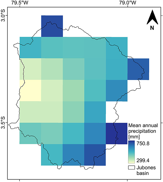
Figure 2. Spatial distribution of GSMaP-NRT data for the Jubones basin.
2.2.2. Geographical information of the Jubones basin
Three main geographical data were used in the methodology: (i) a Digital Elevation Model (DEM), (ii) a soil type map, and (iii) LULC maps. The spatial resolution of the DEM data is 50 m and was freely accessed from Shuttle Radar Topography Mission (SRTM) Global (2013). Whereas, the soil type and LULC maps were obtained from the geoportal of the Ministry of Agriculture, Livestock, Aquaculture and Fisheries (MAGAP) of Ecuador. The corresponding maps have been updated to 2015. Moreover, all geographic information was processed using the software QGIS version 3.18.2 together with the GRASS complement version 7.8.5.
2.2.3. Runoff at the entrance of the MSF hydropower plant
Hourly runoff time series were accessed in real-time through the website of the Corporación Eléctrica del Ecuador (CELEC-SUR), the company that manages of MSF hydropower plant. The gauge station is located at the entrance of the dam of MSF. The mean hourly runoff at the entrance is 53.73 m3/s. We present in Figure 3, the runoff and the mean GSMaP-NRT time series averaged for the entire basin for the study period.
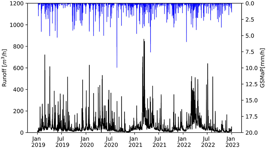
Figure 3. Runoff (black lines) and GSMaP-NRT precipitation (blue lines) time series for the study period (January 2019 to December 2022).
2.3. Methodology
The methodological scheme of this study is presented in the flowchart of Figure 4. This methodology can be divided into four principal steps. The first step involved data processing and the development of referential models; the second step contemplated the development of FE strategies based on geographic data and the SCS-CN method; the third step consisted of the development of specialized models with the FE strategies, and the four-step was the evaluation and comparison between specialized and referential models (without FE strategies). All models were developed for lead times of 1, 6, and 11 h.
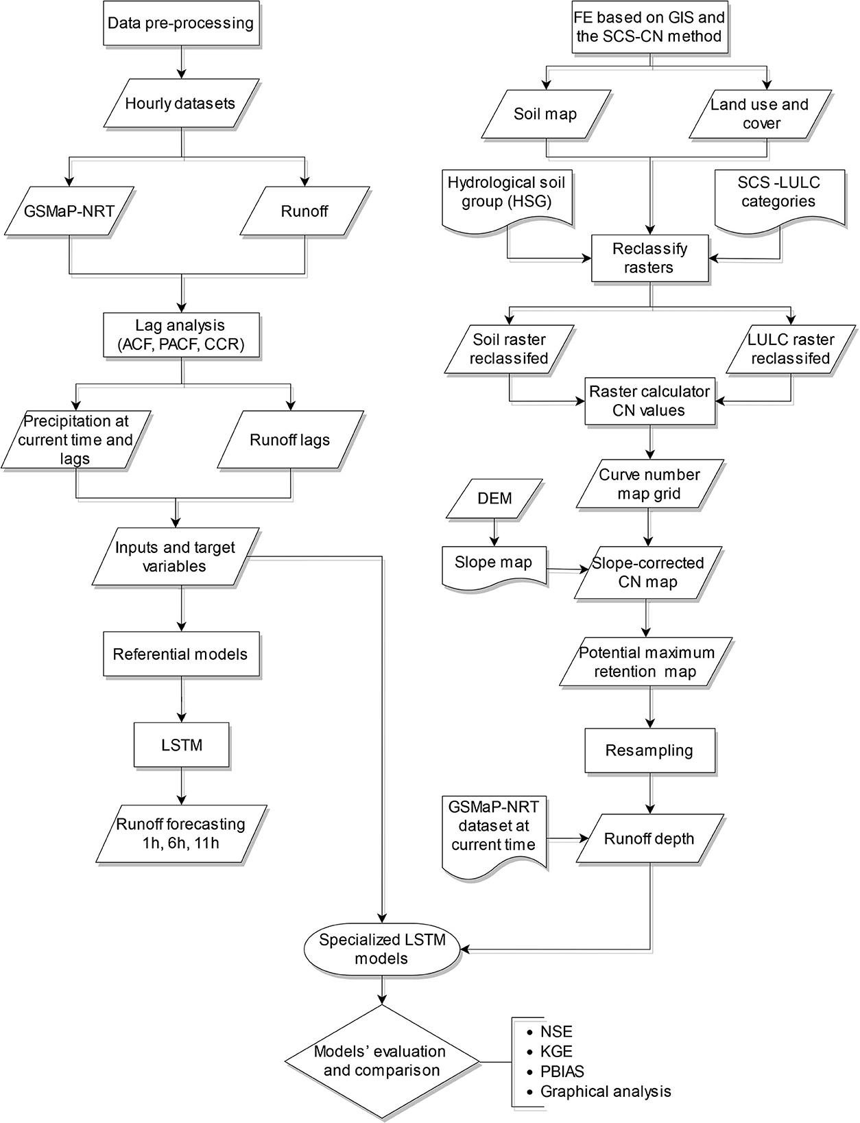
Figure 4. Scheme of the methodology for developing and evaluating referential and specialized runoff forecasting models.
In the first step, we composed the input feature space of the models using current-time and lagged precipitation and runoff information. Runoff-lagged information was determined using the autocorrelation function (ACF) and the partial autocorrelation function (PACF). Whereas, the number of precipitation lags was determined using the cross-correlation function (CCR) between precipitation and the runoff time series. For this, the CCR analysis was applied to the time series of each GSMaP-NRT pixel in the basin. With this information, we developed referential LSTM models for all lead times.
In the second step, we used the geographical data described in Section Materials and methods, which was processed using GIS to derive the necessary parameters for the SCS-CN method. This step involved processing the soil types and LULC maps according to the guidelines of the SCS-CN method. As a result of the map processing, we obtained a CN map, which was then corrected according to a slope map derived from the DEM of the basin. The slope-corrected CN map served to calculate a potential maximum water retention map, and this information was resampled to match the spatial resolution of the GSMaP-NRT product (0.1° x 0.1°). Finally, the hourly runoff depth data was estimated using GSMaP-NRT precipitation data and the resampled map of potential maximum retention.
The third step involved the enrichment of the input feature space of the referential models with the features (pixel-based information) derived from the runoff depth map. Then, in the fourth step, the specialized models were then evaluated and compared to the corresponding referential models using a combination of three efficiency metrics to analyze if the performance improved through the application of FE strategies. In the following, we provide a detailed description of our methodology.
2.3.1. LSTM networks
The LSTM networks proposed by Hochreiter and Schmidhuber (1997) are a type of recurrent neural networks (RNNs) that specifically include memory cells that store information over long periods. The LSTM networks present a cyclical structure that transfers the output of a hidden layer to this same layer to locate features through relationships of the previous time series. The assimilation in each cell can be compared to a state vector in dynamic systems models. For this reason, the LSTM networks have gained significant attention among hydrologists due to the potential for modeling dynamical systems like hydrological basins (Kratzert et al., 2019; Lees et al., 2021).
Similar to RNN, the LSTM structure consists of an input layer, a hidden layer, and an output layer but the difference is that the latter replaces the basic unit with a memory cell that contains three gate functions (input, forget, and output gate). The input gate indicates the information will update the present memory cell state and the new datasets for inputs, the forget gate is the controller for keeping or discarding information, and the output gate controls the output activations.
For the implementation of LSTM models, we used the TensorFlow library (Abadi et al., 2016) for Python version 3.7. The main LSTM hyperparameters are the number of layers, number of units, learning rate, dropout, epochs, batch size, and activation function. We initially set the transfer function of the output layer to linear as suggested by de la Fuente et al. (2019). The architecture and the search space used for the hyperparameterization task are shown in Table 1. For the hyperparameterization task, we employed a randomized-grid search together with a 10-fold cross-validation scheme to avoid overfitting.
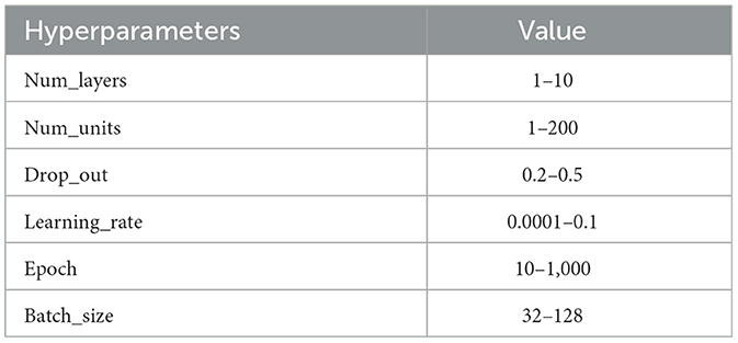
Table 1. Search space of LSTM hyperparameters.
2.3.2. Development of LSTM referential runoff forecasting models
First, we checked the runoff and precipitation data for gaps (<1%) or inconsistent values (<1%). To determine the influence of lagged information on precipitation and runoff, we conducted lag analyses using the ACF, the PACF for runoff, and the CCR function for precipitation. For runoff, the number of lags for the runoff time series was determined by analyzing the ACF and PACF functions using a 95% confidence interval. Whereas, for the precipitation time series, we used the CCR function with a correlation threshold of around 0.2 as recommended by Muñoz et al. (2018). This is because the correlations between non-validated satellite precipitation and runoff tend to be low yet the idea is to rater exploit the spatial variability of this information. For this, the obtained GSMaP-NRT data was clipped to the Jubones basin using the centroids of the cells in the satellite product that match the basin's coordinates. As a result, each cell corresponds to an independent precipitation time series, which can be associated with the Jubones basin as a uniform precipitation network. With this information, we developed LSTM referential models for lead times of 1, 6, and 11 h. Referential models were aimed at providing a benchmark for evaluating the improvement achieved by LSTM specialized models using FE strategies.
2.3.3. Development of specialized LSTM runoff forecasting models
We first implemented the FE strategies based on geographic data and the SCS-CN method, which together with GSMaP-NRT data, served to derive runoff depth in the basin. Second, we used the new features (cells) of the runoff depth map to enrich the input feature space of the referential LSTM models. The LSTM specialized models were developed using enriched input feature space.
2.3.3.1. FE strategies based on geographical information and the SCS-CN method
The first strategy consists in using geographic information (soil, LULC, and slope maps) to derive a CN map of the basin. Then, in the second strategy, the CN map is used to estimate the amount of precipitation that will become direct runoff (runoff depth) from the SCS-CN method and GSMaP-NRT data. This information was derived from the same temporal and spatial resolution of GSMaP-NRT. In summary, the FE strategies proposed in this study consisted in integrating geographical information and the SCS-CN method to derive runoff depth values for enriching the input feature space of LSTM referential models. In the next subsections, we expand on the steps involved.
2.3.3.1.1. Geographical data and reclassification of soil and LULC maps
The soil type and LULC maps were first clipped to the basin and rasterized. For this, we used categorical information on soil and LULC, which were encoded according to each class. Then, these maps were reclassified to the Hydrological Soil Group (HSG) and land use and cover established by the Soil Conservation Service (Mishra and Singh, 2003; Natural Resources Conservation Service, 2004). The HSG is divided into four principal groups corresponding to A, B, C, and D (Mishra and Singh, 2003). Group A includes soils with a high infiltration capacity and a high rate of water transmissions such as sands or gravels. Soils in group B have moderate infiltration rates as their rate of water transmission, like soils with moderately fine to coarse textures. In group C, soils exhibit a low infiltration rate and poor water transmission when completely saturated, for example, soils with moderately fine to fine textures. Finally, group D represents soils with very low infiltration rates and very low rates of water transmission through their layers.
For the LULC classification, there are some adaptations from the original method (Mishra and Singh, 2003) since it was developed for small agricultural catchments. Thus, four principal classes were generated for the basin, which are agricultural, urban, forest, and wetlands/water. Having these categories for soils and LULC, the original raster maps were reclassified into these new simplified classes, and to have a consistent raster operation, both raster maps were resampled into the same cell size (0.1° x 0.1°). These operations were carried out with QGIS software.
2.3.3.1.2. Antecedent moisture condition
The Antecedent Moisture Condition (AMC) is related to the soil moisture condition before the runoff generation, and according to the NEH-4 is classified into three principal classes based on the 5-day antecedent rainfall. AMC I considers that the soils are practically dry, AMC II represents the average conditions of moisture, and finally, AMC III represents the condition where soils are in a constant saturation state (Mishra and Singh, 2006). The original SCS-CN method constructed this classification based on the dormant and growing season and their effects on evapotranspiration (Mishra and Singh, 2003). For this study, the AMC II was selected according to the recommendations of the literature review for ungauged heterogeneous basins (Mishra and Singh, 2006; Lal et al., 2019).
2.3.3.1.3. Curve number estimation map
To determine the most appropriate CN, we looked at the tables from the NEH-4. The CN is a dimensionless parameter with values between 0 and 100, where 0 represents no runoff generation and the maximum value of 100 indicates that all precipitation becomes runoff. For this, a raster operation with the HSG and LULC reclassified maps of the Jubones basin was performed. The operation consisted of assigning the value of CN according to the reclassification classes described before. In this case, each cell of the resulting raster map of CN constitutes a hydrological unit with a specific CN parameter according to its soil and LULC information.
2.3.3.1.4. CN correction based on slope
The SCS-CN method was designed for basins with an average slope of 5%. Therefore, multiple studies have evaluated the effectiveness of this method in steep slope basins and recommended corrections to the original formulas to improve the representation of slope in runoff response (Ajmal et al., 2020; Ansari et al., 2020; Sharma et al., 2022). We employed, the equation proposed by Ajmal et al. (2020) for steep-slope basins, varying from 7.5 to 53.5%. The corresponding equation 1 is described below:
Where CNII∝ is the slope-adjusted CN for the average antecedent moisture condition, CNIII is the CN for saturated moisture conditions, and ∝ corresponds to the average slope of the basin area [m/m]. Through the conversion of CNIII to CNII suggested by Mishra et al. (2008), equation 1 could also be represented as equation 2:
Thus, in this equation, the CN corrected by slope is in direct function of the CN with average antecedent moisture condition for the basin. To apply this correction, first, the slope map of the Jubones basin was derived from the DEM with GIS operations. Then, equation 2 was applied to the CN map using the slope map values in the raster calculation.
2.3.3.1.5. Potential maximum water retention map
To determine the amount of potential maximum water retention (S), we used equation 3 below.
Where the CN is the parameter determined before. This value can theoretically vary between zero to infinite. This equation was applied to each cell of the CN slope-corrected map with the raster calculator.
2.3.3.1.6. Resampling of potential maximum water retention map
The resulting potential maximum water retention map was resampled to the spatial resolution of the GSMaP-NRT product (0.1° x 0.1°) to calculate the runoff depth using the precipitation time series of each cell. The interpolation method selected to resample was a bilinear interpolation as suggested by Chao et al. (2022) for continuous hydrological variables. In the bilinear interpolation, each cell in the new raster is assigned an average value based on the four nearest original cells. As a result, the averaging is linear in both the horizontal and vertical directions. This operation was performed using a raster map of GSMaP-NRT precipitation data to acquire its same spatial resolution for the new map of potential maximum retention (S).
2.3.3.1.7. Runoff depth using GSMaP-NRT data
The estimation of runoff depth derived from the SCS-CN method is based on a water balance concept together with two hypotheses. The first hypothesis implies that the amount of rainfall that becomes direct surface runoff depends on the amount of rainfall that infiltrates the soil and the potential maximum retention capacity of the soil. The second hypothesis assumes that the amount of water lost to initial abstraction is proportional to the potential maximum retention capacity of the soil (Mishra and Singh, 2003). These hypotheses are equated to form the basic empirical relation of the SCS-CN method and it is presented in equation 4:
Where F is the actual retention, S is the potential maximum retention as mentioned before, Q is the accumulated runoff depth, P is the accumulated precipitation and Ia is the initial abstraction. The basic water balance equation 5 is:
Combining equations 4 and 5 results in equation 6:
The relationship to estimate the value of Ia is 0.2S according to a regression analysis based on continuous experiments in multiple basins (Mishra and Singh, 2003). This initial abstraction also is represented as Ia = λS, and λ = 0.2 is recommended for general use (Al-Ghobari et al., 2020). Thus, combining these relationships, the resulting equation 7 is the precipitation-runoff relationship used in the SCS-CN method.
Equation 7 allows us to estimate the runoff depth [mm] from precipitation and the potential maximum retention. The runoff depth for the Jubones basin was calculated for each one of the cells of precipitation using the GSMaP-NRT data at current time. Therefore, given equation 7, the resampled map of potential maximum retention (S), and the GSMaP-NRT precipitation datasets, the runoff depth values were derived from each time step at an hourly scale.
2.3.3.2. Specialized LSTM runoff forecasting models set up
The new inputs derived from the SCS-CN method using terrain information of the Jubones basin and precipitation data from GSMaP-NRT with lags were added to the new feature space for the runoff forecasting LSTM models (referential) for each lead time.
2.3.4. Models' evaluation and comparison
We evaluated the forecasting efficiencies of LSTM referential and specialized models using the most-employed efficiency metrics in hydrological applications (Contreras et al., 2021; Bhusal et al., 2022; Chen et al., 2022; Li et al., 2022). These are the Nash-Sutcliffe efficiency (NSE) (Nash and Sutcliffe, 1970), the Kling-Gupta efficiency (KGE) (Gupta et al., 2009), and the Percent Bias (PBIAS). The NSE is usually applied to measure the overall model accuracy and is less sensitive to high extreme values due to underestimating runoff peaks (Gupta et al., 2009). The KGE addresses the shortcomings of NSE (Knoben et al., 2019) and is nowadays, increasingly used for the evaluation of hydrological models due to the incorporation of its three components (correlation, bias, and the relative variability of flows) (Gupta et al., 2009; Li et al., 2022) and improve the evaluation for runoff peaks. The PBIAS is a measure that determines the tendency of simulated values to deviate from observed values. In Table 2 the equations used for each metric are presented.
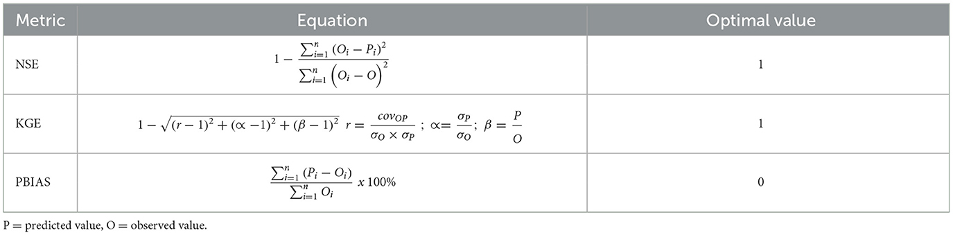
Table 2. Metrics used for evaluation of models.
For evaluation, in terms of NSE, according to the guidelines for hydrological model evaluation proposed by Moriasi et al. (2007), values upper than 0.75 are considered very good. According to the KGE, it allows the evaluation of error (r), the relative variability of observed and predicted runoff values (∝), and the bias (β). For the PBIAS metric, between 0 and 10% values, models are considered to have a very good adjustment in comparison with observed data, with minimum overestimations or underestimations (Gupta et al., 1999). Also, the performance of these models was evaluated through graphical inspection with hydrograph plots and cumulative runoff volumes for a better interpretation of the fit between the observed and forecasting runoff values.
3. Results
In this section, we first present the obtained composition of the input feature space for the LSTM referential models. Second, we show the corresponding maps derived during the FE implementation thought the SCS-CN method process until obtaining runoff depth maps for the basin. Lastly, we present the evaluation of the LSTM specialized models and a comparison with the corresponding referential models.
3.1. Development of LSTM referential runoff forecasting models
Figures 5A, B shows the results of the ACF and PACF analyses. For the ACF with a 95% confidence interval, we found a significant correlation up to around 700 lags, which corresponds to 29 days. The correlation decayed rapidly after the highest correlation at first lag which indicates an autoregressive process. On the other hand, the PACF with a 95% confidence interval revealed a significant correlation up to lag 8, and showed a rapid decay of PACF, confirming the presence of an autoregressive process in the runoff data. Based on these analyses, we decided to include 8 lags (hours) of runoff to the input feature space of the forecasting models.
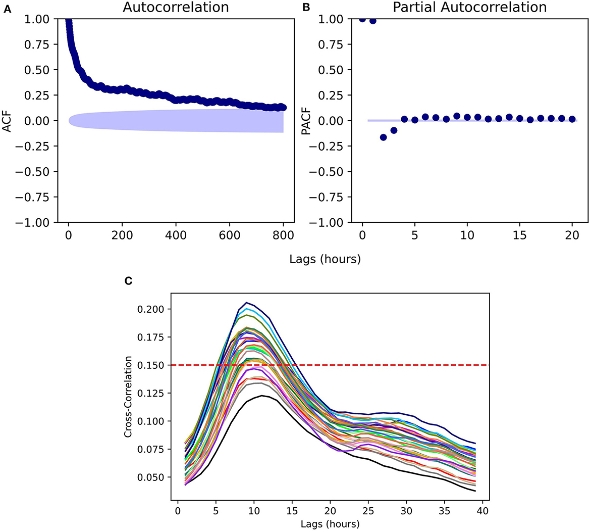
Figure 5. (A) Autocorrelation function (ACF) and (B) partial autocorrelation function (PACF) for runoff values at the entrance of the MSF hydropower plant. (C) CCR between GSMaP-NRT precipitation data and runoff. The horizontal red line at a cross-correlation of 0.15 and each curve represents the pixel of GSMaP-NRT data for the Jubones basin.
In addition, Figure 5C presents the CCR plot for each one of the 29 pixels of the GSMaP-NRT in the basin when correlated to the runoff time series. Overall, we determined 11 precipitation lags using the correlation threshold of 0.15. The number of precipitation lags matches the concentration time of the catchment, which was estimated as 11 h in the study of Muñoz et al. (2023). The use of 11 precipitation lags and the precipitation at the current time for each one of the 29 pixels in the basin, together with eight runoff lags and the runoff data resulted in an input feature space dimension of 356 features. The number of instances was 35,053 for the study period.
3.2. Development of specialized LSTM runoff forecasting models
In this subsection, we present the results of the FE strategies using geographic data and the SCS-CN method. Then, the set-up of specialized LSTM models with these strategies by using FE-based inputs, and finally, the evaluation and comparison of referential vs. specialized LSTM models.
3.2.1. Feature engineering strategies based on geographic data and the SCS-CN method
3.2.1.1. Soil and LULC reclassification maps
The reclassification process for soil orders of the Jubones basin was performed according to the soil texture assigned to each HSG. Results showed the predominance of soils belonging to group C, which covers 60% of the basin. These soils are Alfisol and Inceptisol which are characterized by higher clay content with moderate to lower permeability. Inceptisol is characterized by a moderate to a low rate of water transmission and the presence of sandy clay loam and silts, with a high sand content and usually porous materials used to be present due to volcanic formation (Larson and Padilla, 1990; Riveras-Muñoz et al., 2022). The dominance of soils group C was followed by group B, with Entisol representing 25% of the total area of the basin. This was followed by group B, which has a loamy-sand to loamy clay and a moderate permeability (Mejía-Veintimilla et al., 2019). Finally, Histosol, Mollisol, and Vertisol were classified in group D with <15% of the basin area. Regarding the classification of the LULC, the herbaceous and shrub vegetation (46%), pastureland (28%), and paramo (15%) were the most representative LULC classes in the Jubones basin. For the application of the SCS-CN method, the forest and agricultural and cropped land were the most representative classes in the basin covering 99% of the area. With the results, we present in Figure 6 the spatial distribution of soil and LULC classification and their respective reclassification process. In the Supplementary material, we show two tables summarizing the reclassification of the soil order map to the Jubones basin into the HSG and the LULC reclassification.
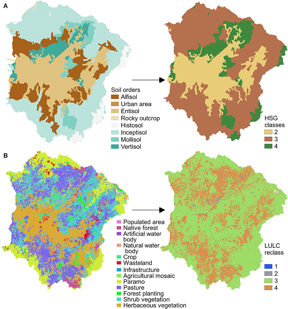
Figure 6. (A) Soil and (B) LULC maps and their corresponding reclassification.
3.2.1.2. Curve number map and correction based on slope
The CN map was derived from the established tables of NEH-4, according to the reclassified maps of soil and LULC, and considering the AMC II (average conditions of soil moisture). The CN values determined for the Jubones basin range from 58 to 100 (Figure 7A). The highest CN values indicate that a larger proportion of rainfall will become runoff rather than being absorbed into the soil (less infiltration capacity). The CN value of 100 indicates that all rainfall will run off the surface, and no infiltration will occur, as is the case with water bodies. These highest values are found in the zone of HSG D, which is characterized by low infiltration rates and high runoff potential. These soils are typically composed of heavy clay or fine-grained soils, which have low permeability and high water-holding capacity, such as Histosols. The lowest values represent moderate infiltration rates. These values were found in hydrological soil group B which corresponds to soils with moderate runoff potential due to the lack of soil development and low organic matter content. To the CN map, the slope correction was applied (Figure 7C) using the equation 2 and the slope map (Figure 7B). With the slope correction, high CN values became higher, while low values were reduced. This indicates that the impact of slope on runoff generation is significant within the basin, largely due to the complex topography. In particular, areas with steep slopes exhibited higher CN values, as steeper slopes tend to produce greater amounts of runoff.
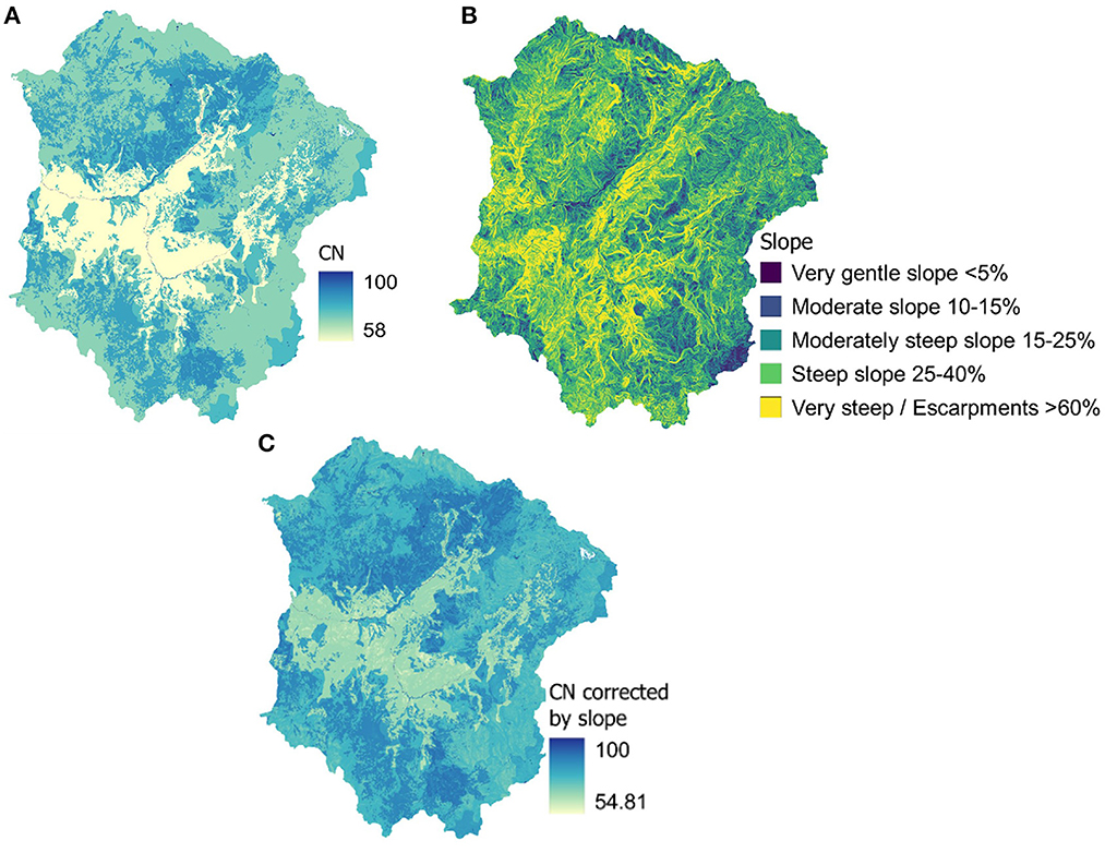
Figure 7. (A) Curve number map in the Jubones basin, (B) slope map, and (C) slope-corrected CN map.
3.2.1.3. Potential maximum water retention map
The slope-corrected CN map was used as the input for the calculation of the maximum potential water retention using equation 3. As shown in Figure 8A, the values range from 0 to 200, which is the result of the high variability of CN values and the combination of soil, LULC, and slope features. Generally, higher values indicate that the soil has a greater capacity to hold water and mainly represent infiltration occurring after runoff has started given the CN values. The values equal to 0 represent completely impermeable surfaces and in this case, represent water bodies due to the absence of soil. Then, this map was resampled with the bilinear interpolation method to the same spatial resolution as GSMaP-NRT (0.1° x 0.1°) for appropriate runoff depth estimation. The resampled map (Figure 8B) retained the spatial distribution of the potential water retention map, with the highest values located in the center near the outlet of the basin, whereas the lowest values were found in the northern part of the basin.
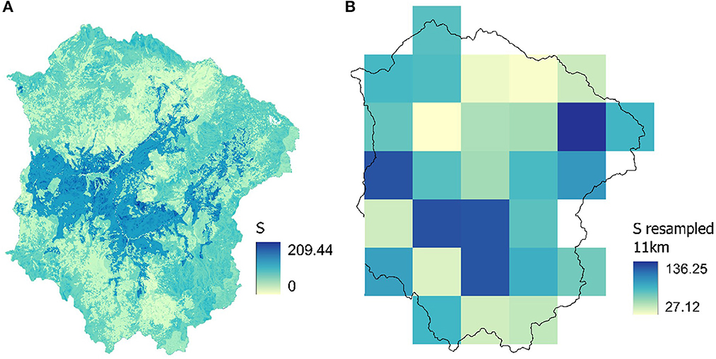
Figure 8. (A) The potential maximum water retention map and the (B) resampled map.
3.2.1.4. Runoff depth time series
The precipitation data series obtained from GSMaP-NRT, and the resampled potential maximum water retention map were used as inputs to calculate the hourly runoff depth using equation 7. The runoff depth was estimated for each one of the 29 pixels of the GSMaP-NRT data pixel. The spatial distribution of the mean runoff depth estimated for the Jubones basin is shown in Figure 9, with values ranging from 2.78 to 5.18 on an hourly scale for the study period.
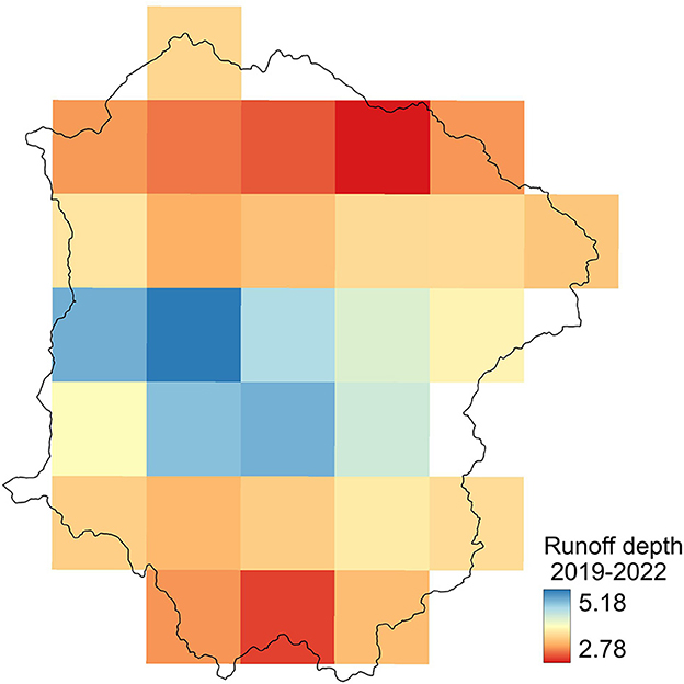
Figure 9. Mean runoff depth map for the study period (Jan/2019- Dec/2022).
3.2.2. Set-up of specialized LSTM models
We used new features derived from the runoff depth map, which corresponds to the difference between the amount of precipitation that fell on a given area (in this case, the pixel area of approximately 121 km2) and the amount of water that infiltrates into the soil and is affected by soil type, land cover, and slope. Thus, in the feature space of the referential models, 29 new inputs were aggregated for the performance of the specialized models.
To improve the representation of these new features in the feature space, a Principal Component Analysis (PCA) was applied to the precipitation inputs (348 inputs) for reducing the dimensionality while retaining as much of the original information as possible. We retained 80% of the explained variance with seven components from the precipitation lags to have a minor number of inputs in contrast with the inputs derived from FE strategies. This percentage of variance was determined on a trial-and-error basis for maximizing forecasting efficiencies.
The feature space was composed of the PCA-derived features of precipitation (7), the runoff lags (8), and the features from the FE strategies described before (29). The hyperparameters used to tune the specialized models were the same as those detailed in Table 1. In Supplementary material we present a table with the hyperparameters used for these models.
3.3. Evaluation and comparison of LSTM referential and specialized models
Table 3 shows the efficiency metrics of both the referential and specialized LSTM models for the testing period. For the 1 h forecasting, the LSTM specialized models achieved higher efficiencies with all efficiency metrics when compared to referential models. We found efficiency improvement in the specialized models when compared to the referential ones for all efficiency metrics and for all lead times. For instance, for the 1 h lead times, the NSE values increased from 0.9 to 0.93, the KGE values increased from 0.94 to 0.97, and the PBIAS decreased from 0.82 to 0.35 which indicates a better approximation to 0.
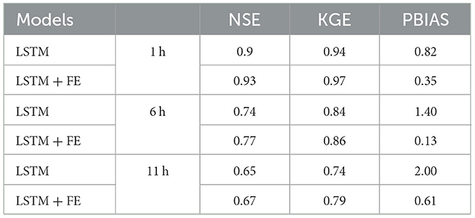
Table 3. Comparison of efficiencies between referential and specialized models using FE strategies, and across lead times.
We found the same pattern for the lead times of 6 and 11 h. Moreover, all the efficiency values in terms of the NSE, the KGE, and the PBIAS for the LSTM specialized models lay within the range considered a very good (1 and 6 h) and good (11 h) model performance according to the criteria of Moriasi et al. (2007).
We also present the efficiencies of the referential and specialized LSTM modes in the scatter plots of Figure 10. In this figure, specialized model forecasts (gray dots) appeared to have less dispersion and were closer to observations in comparison with the forecasts obtained with referential models (black dots). This is especially true for runoff magnitudes up to 200 m3/s. On the contrary, for more extreme runoffs (>200 m3/s), there is no significant improvement of the LSTM specialized models when compared to the referential ones. This indicates that the developed specialized models are good at estimating runoff values close to the mean (53 m3/s), up to a threshold of value 200 m3/s. Although the differences were not considerably higher, we rather demonstrated the possibility to assimilate geographic data and the derived runoff depth features in the pursuit of improved runoff forecasts. We are aware that it is still research for achieving further improvements, principally for extreme runoff events, where information other than precipitation such as soil moisture dynamics is crucial.
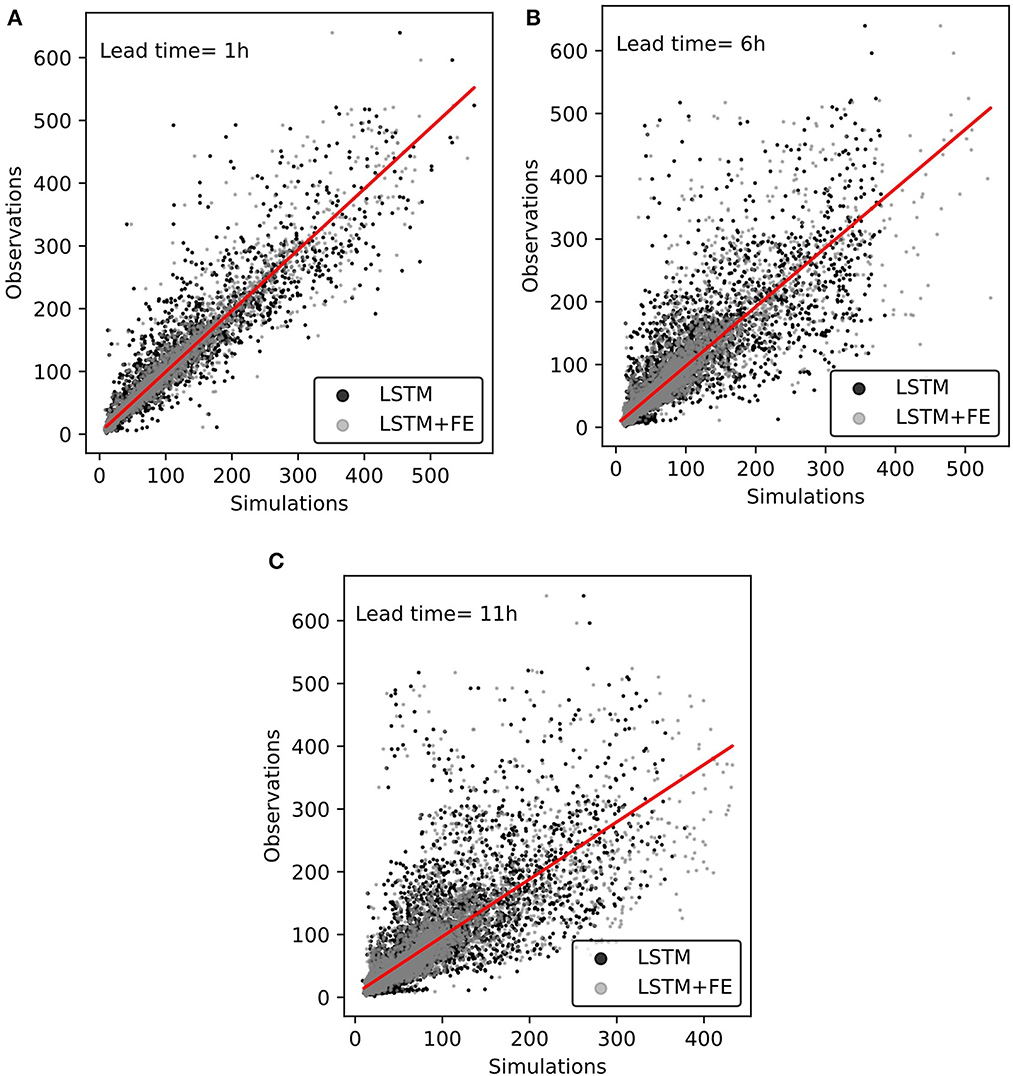
Figure 10. Scatter plots of runoff forecasting models for referential and specialized models. (A) 1 h-lead time, (B) 6 h-lead time, and (C) 11 h-lead time.
To show the performance of LSTM models, we provide in Figure 11 the results of LSTM models for the lead times of 6 and 11 h, which showed the greatest improvements when LSTM specialized models were compared to the referential models. For this, we highlight in a red rectangle the period from February to May, which presented runoff values up to 500 m3/s. Overall, the ability of LSTM models to forecast runoff decreased as the lead time increased. It can be observed that the specialized model for the 6 and 11 h achieved better approximations of the observations when compared to their corresponding referential models.
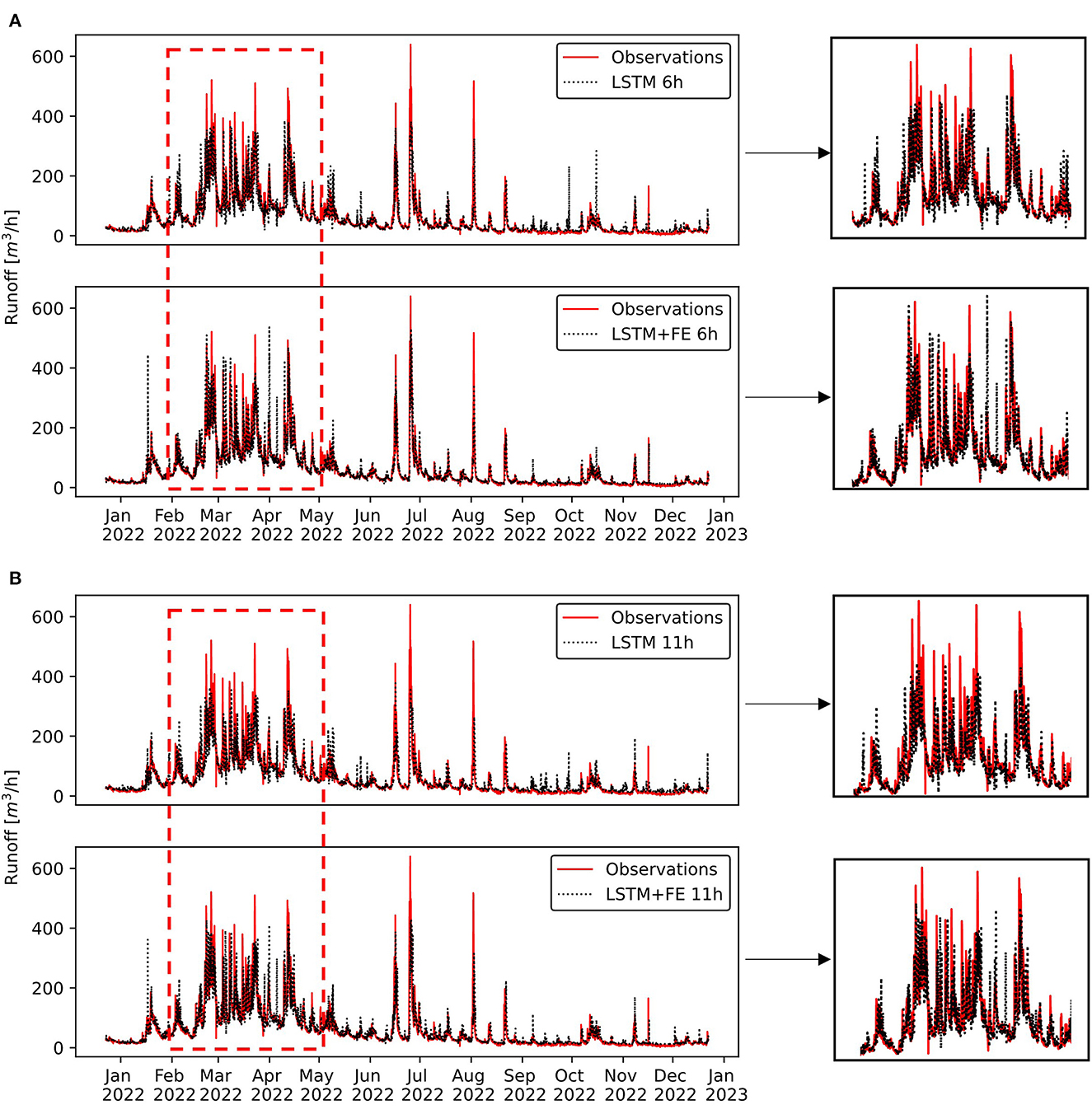
Figure 11. Results for the validation period (January 2022 to December 2022) of referential and specialized LSTM models for lead times of (A) 6 and (B) 11 h.
In addition, a graphical representation of the cumulative runoff values for the validation period has been provided in Figure 12. This figure served to compare and contrast the water volumes obtained from the developed forecasting models. In this figure, it is clear that LSTM specialized models perform better than referential models in predicting observed data, as their curves are closest to the observed values. This is because LSTM specialized models have lower PBIAS values, indicating lower underestimations when compared to the LSTM referential observed models. Therefore, specialized models are more effective in accurately predicting the amount of runoff volume compared to referential models.
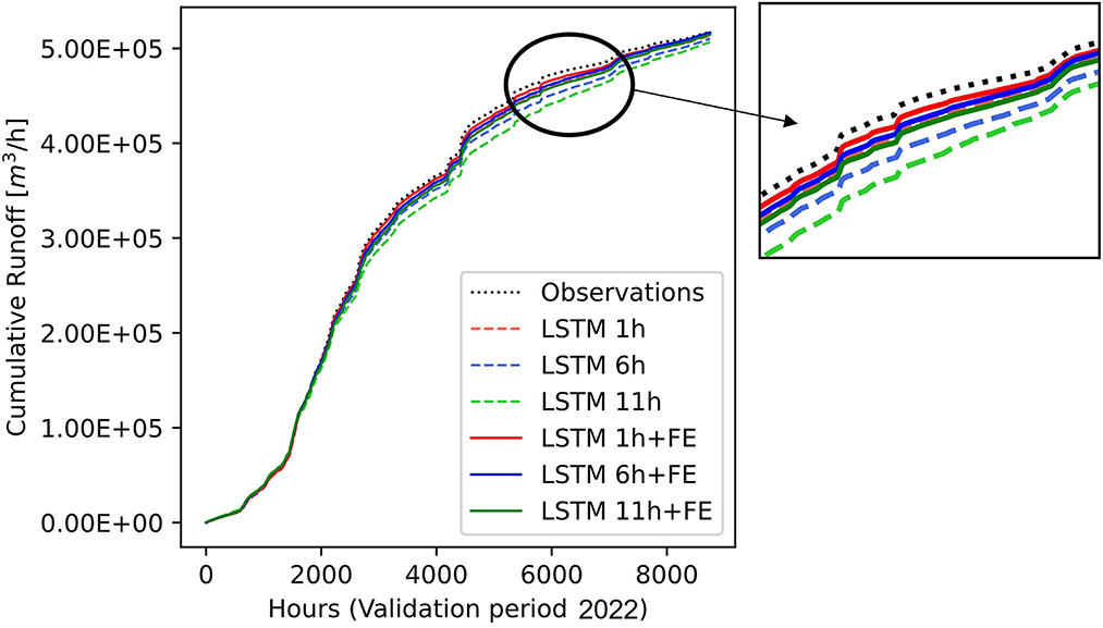
Figure 12. Comparison of cumulative runoff values for referential and specialized models.
4. Discussion
This study proposes a methodology for improving the efficiency of LSTM runoff forecasting models by developing specialized models using GIS-based FE strategies and the SCS-CN method in a complex basin of Ecuador. We aimed to evaluate the effectiveness of specialized models by comparing them with conventional LSTM models. We demonstrated the usefulness and limitations of the proposed LSTM specialized models across increasing lead times. The study findings offer valuable insights into the potential of the LSTM models for runoff forecasting and highlight the significance of using GIS-based FE strategies and the SCS-CN method in enhancing the accuracy of the models.
The results of this study showed that for all runoff forecasting lead times, FE strategies improve the efficiency metrics in comparison with the referential models. This indicates that the proposed strategies using terrain information and the inclusion of hydrological information were effective for a complex mountain basin through the use of LSTM models. Moreover, even though we developed models with a relatively short data period, we obtained promising efficiencies when compared to other studies using much longer data records. Despite the limitations of this study, the proposed methodology can serve as a valuable guideline for developing runoff forecasting models in other basins and regions where data limitations have previously made it impossible. The use of GIS-based FE strategies and the SCS-CN method in conjunction with LSTM models has the potential to enhance the accuracy of runoff forecasting and enable more effective water resource management in various regions. Further research and development in this area can lead to improved methodologies and greater applicability of the models for runoff forecasting in diverse hydrological systems.
The efficiency of the developed LSTM specialized models achieved NSE values of 0.93, 0.77, and 0.67 for lead times of 1, 6, and 11 h, respectively. These results are comparable to the results of Zhou et al. (2023), who used ground precipitation for a 1,758 km2 basin. In that study, the authors obtained NSE values of 0.95 and 0.78 for lead times of 1 and 6 h, respectively. In comparison with the information used in Zhou et al. (2023), in our study area, one of the principal challenges (limitations) was the lack of ground precipitation information for forecasting modeling. However, the GSMaP-NRT data in conjunction with the FE strategies applied to the runoff forecasting models allowed for achieving very good efficiencies in terms of NSE according to Moriasi et al. (2007) due to these limitations.
Our results can also be compared with the study of Li et al. (2022), who used a combined approach of LSTM and Convolutional Neural Networks (CNN) to assimilate spatial patterns between precipitation radar data and long-term runoff data. For this, the authors selected high and low water periods in a period study of 15 years. The authors found NSE values of 0.78 for the high-water period and 0.81 for the low-water period, respectively. If we compare those results with our results (NSE 1 h = 0.93, KGE 1 h = 0.97, NSE 6 h = 0.77, KGE 6 h = 0.86), we can conclude that some clear advantage of our models is the reduction of data-driven model complexity, the inclusion of hydrological concepts through the FE applied, and the possibility to implement our models for real-time operation since we employed near-real-time satellite precipitation products (SPPs). This opens the path for replicating this study in other basins/regions experiencing a lack of ground-based precipitation monitoring.
Another comparison can be done with the study Mejía-Veintimilla et al. (2019), who used the SCS-CN method in the Runoff Prediction Model and obtained NSE values of 0.82 using a physically-based model fed by high-resolution meteorological radar data for a small area (5 km2) Andean basin. Although the authors employed physically-based models and more precise precipitation information, the NSE values derived from our models demonstrate the utility of our methodology for developing forecasting models in precipitation-ungauged basins through the exploitation of non-validated satellite precipitation products. This finding matches with the insights provided in the study of Kratzert et al. (2019), which indicates that physically based models and data-driven models are both effective for predicting runoff. However, data-driven models have the added advantage of being able to transfer model parameters to other ungauged basins that share similar biophysical characteristics. This allows for a more efficient and cost-effective approach to runoff forecasting in ungauged basins, where ground observations are often limited or unavailable.
Furthermore, the efficiency evaluation of our models indicated that the main differences between the LSTM specialized, and referential models were found in the calculated PBIAS, a critical parameter for preventing underestimation of forecasted runoff values. This finding is particularly significant for closing hydrological balances, given that the LSTM specialized models produced accumulated water amounts that were close to the observed runoff values. These results suggest that it may not be necessary to add mass conservation equations to LSTM models, as concluded by Frame et al. (2022) who found that adding mass balance constraints actually reduced the model's skill during extreme events. These findings contribute to the ongoing debate about the most effective ways to incorporate physical constraints into data-driven models and can guide future research in this area.
Another important finding is related to the practical and simple method for improving the runoff forecasting models using the SCS-CN method which could be derived from open-source geographical information and GIS tools. The inclusion of information about the soil types, LULC, and topography, among other features related to runoff generation, showed important improvements in hydrological modeling and runoff forecasting (Mahmoud, 2014; Asadi et al., 2019; Huang et al., 2019; Meresa, 2019; Kwon et al., 2020). Here, the performance of the specialized models reflected the importance of the inclusion of this information in an interpretable way for data-driven models, in this case through the SCS-CN method. However, according to the limitations of the SCS-CN method due to is considered under an empirical approach, its application in complex basins should be reviewed to avoid inconsistencies. Furthermore, future research can be focused on improving the inputs for developing these FE strategies proposed with more recent and better resolution of geographical information.
Finally, the use of satellite precipitation data continues to be an important alternative for precipitation-ungauged systems, and thus exploiting additional SPPs is a promising future direction for overcoming detection failures in a given SPP. However, in addition to the forecasting lead time, consideration of the latency time of the SPP employed (5 h in the case of the GSMaP-NRT product) must be taken into account since this represents an additional source of uncertainty, especially when relying on physically-based hydrological models. This is evidenced in the study of Llauca et al. (2021), where the uncertainty arising from the latency of SPP led to the finding that SPPs with shorter latency times do not guarantee effectiveness in runoff modeling when using a reservoir-based hydrological model. Therefore, this highlights another compelling reason for employing deep learning techniques like LSTM neural networks, which have the capability to effectively relate available precipitation data (accounting for lead time and latency time) to predict future runoff. Utilizing more than one SPP using a modular approach for SPP data usage, as described in Muñoz et al. (2023), can lead to a more accurate spatial characterization of precipitation and therefore more accurate runoff forecasts. This approach could be particularly useful in areas with complex terrain, where precipitation patterns can vary greatly across short distances.
5. Conclusions
This study aimed to improve the efficiency of the runoff forecasting model by developing FE strategies based on geographic data and the SCS-CN method in a 3,340 km2 precipitation-ungauged basin representative of complex hydrological systems in the Andes of Ecuador. We proposed a stepwise methodology for developing and evaluating forecasting models that exploit readily available satellite precipitation data, assisted by FE strategies for LSTM networks. The developed models accounted for lead times of 1, 6, and 11 h to enable near-real-time forecasting, flash floods, and a lead time equal to the concentration-time of the basin, respectively. The success of developing accurate short-term runoff forecasting models using LSTM networks can be first attributed to their ability to capture temporal dependencies between features. Second, the application of FE strategies, including the incorporation of thematic maps such as soil types, LULC, slope information, and the SCS-CN method, was found to be effective for integrating process-based hydrological knowledge into LSTM models.
The NSE values across increasing lead times varied from 0.93 to 0.67 for lead times between 1 and 11 h, respectively. The KGE values were higher than NSE values for all lead times, which demonstrated that models are also able to forecast peak runoff values. Although this study did not aim to outperform physically-based models, the obtained efficiencies are comparable to that modeling approach and other studies employing higher resolution data such as ground-based weather radars and rain gauges. Thus, this study proposes a solution for the cases of precipitation-ungauged basins and has the potential to be replicated in other hydrological systems in the Andes and/or regions where geographic data is available.
We recommend future research focused on assessing the developed methodology with other deep learning techniques such as convolutional neural networks for adding spatial patterns that can represent the runoff processes generation by regions. Additionally, we recommend exploring the use of additional precipitation data sources, such as soil moisture and vegetation indices, to further improve runoff forecasting performance in complex mountain basins. Ultimately, the development of accurate and efficient runoff forecasting models using machine learning and FE strategies can greatly benefit the management of water resources in mountainous regions.
Data availability statement
The data analyzed in this study is subject to the following licenses/restrictions: we employed datasets from two variables, precipitation and runoff. Precipitation data is freely available from the portal of the Global Satellite Mapping of Precipitation (https://sharaku.eorc.jaxa.jp/GSMaP/guide.html). Whereas, runoff was obtained from the CELEC-SUR company in Ecuador, and is available only upon request. Requests to access these datasets should be directed to informacion@celec.gob.ec.
Author contributions
MM and PM contributed to the conception and design of the study, methodology, and writing. GC, DM, and ES contributed to methodology and supervision. RC contributed to funding acquisition, methodology, project administration, resources, supervision, and writing—review and editing. All authors contributed to the article and approved the submitted version.
Funding
This research was funded by the Vice-rectorate for Research of the University of Cuenca (VIUC) and the Corporación Eléctrica del Ecuador-Unidad de Negocio Sur (CELEC-SUR) through the project: Data fusion of remote sensing products and machine learning feature engineering strategies for near-real time runoff forecasting. Our thanks go to these institutions for their generous funding.
Acknowledgments
The authors would also like to thank the editors and reviewers for their constructive comments that are greatly contributive to enriching the manuscript.
Conflict of interest
The authors declare that the research was conducted in the absence of any commercial or financial relationships that could be construed as a potential conflict of interest.
Publisher's note
All claims expressed in this article are solely those of the authors and do not necessarily represent those of their affiliated organizations, or those of the publisher, the editors and the reviewers. Any product that may be evaluated in this article, or claim that may be made by its manufacturer, is not guaranteed or endorsed by the publisher.
Supplementary material
The Supplementary Material for this article can be found online at: https://www.frontiersin.org/articles/10.3389/frwa.2023.1233899/full#supplementary-material
References
Abadi, M., Agarwal, A., Barham, P., Brevdo, E., Chen, Z., Citro, C., et al. (2016). “TensorFlow: large-scale machine learning on heterogeneous distributed systems,” in OSDI'16: Proceedings of the 12th USENIX conference on Operating Systems Design and Implementation, 265–283.
Adnan, R. M., Petroselli, A., Heddam, S., Santos, C. A. G., and Kisi, O. (2021). Short term rainfall-runoff modelling using several machine learning methods and a conceptual event-based model. Stochast. Environ. Res. Risk Assess. 35, 597–616. doi: 10.1007/s00477-020-01910-0
Ajmal, M., Waseem, M., Kim, D., and Kim, T. W. (2020). A pragmatic slope-adjusted curve number model to reduce uncertainty in predicting flood runoff from steep watersheds. Water 12:1469. doi: 10.3390/w12051469
Al-Ghobari, H., Dewidar, A., and Alataway, A. (2020). Estimation of surface water runoff for a semi-arid area using RS and GIS-Based SCS-CN method. Water 12, 1–16. doi: 10.3390/w12071924
Ansari, T. A., Katpatal, Y. B., and Rishma, C. (2020). A Historical Review of Slope Based SCS Method and its Effect on CN and Runoff Potential Globally, p. 1–7. doi: 10.20944/preprints202010.0024.v1
Asadi, H., Shahedi, K., Jarihani, B., and Sidle, R. C. (2019). Rainfall-runoff modelling using hydrological connectivity index and artificial neural network approach. Water 11:212. doi: 10.3390/w11020212
Bhusal, A., Parajuli, U., Regmi, S., and Kalra, A. (2022). Application of machine learning and process-based models for rainfall-runoff simulation in dupage river basin, Illinois. Hydrology 9:117. doi: 10.3390/hydrology9070117
Campozano, L., Mendoza, D., Mosquera, G., Palacio-Baus, K., Célleri, R., and Crespo, P. (2020). Wavelet analyses of neural networks based river discharge decomposition. Hydrol. Process. 34, 2302–2312. doi: 10.1002/hyp.13726
Chao, L., Zhang, K., Wang, S., Gu, Z., Xu, J., and Bao, H. (2022). Assimilation of surface soil moisture jointly retrieved by multiple microwave satellites into the WRF-Hydro model in ungauged regions: towards a robust flood simulation and forecasting. Environ. Model. Softw. 154:105421. doi: 10.1016/j.envsoft.2022.105421
Chen, X., Huang, J., Wang, S., Zhou, G., Gao, H., Liu, M., et al. (2022). A new rainfall-runoff model using improved LSTM with attentive long and short lag-time. Water 14:697. doi: 10.3390/w14050697
Clark, M. P., Bierkens, M. F. P., Samaniego, L., Woods, R. A., Uijlenhoet, R., Bennett, K. E., et al. (2017). The evolution of process-based hydrologic models: historical challenges and the collective quest for physical realism. Hydrol. Earth Syst. Sci. 21, 3427–3440. doi: 10.5194/hess-21-3427-2017
Contreras, P., Orellana-Alvear, J., Muñoz, P., Bendix, J., and Célleri, R. (2021). Influence of random forest hyperparameterization on short-term runoff forecasting in an andean mountain catchment. Atmosphere. 12:238. doi: 10.3390/atmos12020238
de la Fuente, A., Meruane, V., and Meruane, C. (2019). Hydrological early warning system based on a deep learning runoff model coupled with a meteorological forecast. Water 11:1808. doi: 10.3390/w11091808
Falchetta, G., Kasamba, C., and Parkinson, S. C. (2020). Monitoring hydropower reliability in Malawi with satellite data and machine learning. Environ. Res. Lett. 15. doi: 10.1088/1748-9326/ab6562
Fang, Z., Wang, Y., Peng, L., and Hong, H. (2021). Predicting flood susceptibility using LSTM neural networks. J. Hydrol. 594:125734. doi: 10.1016/j.jhydrol.2020.125734
Frame, J. M., Kratzert, F., Klotz, D., Gauch, M., Shalev, G., Gilon, O., et al. (2022). Deep learning rainfall-runoff predictions of extreme events. Hydrol. Earth Syst. Sci. 26, 3377–3392. doi: 10.5194/hess-26-3377-2022
Gupta, H. V., Kling, H., Yilmaz, K. K., and Martinez, G. F. (2009). Decomposition of the mean squared error and NSE performance criteria: implications for improving hydrological modelling. J. Hydrol. 377, 80–91. doi: 10.1016/j.jhydrol.2009.08.003
Gupta, H. V., Sorooshian, S., and Yapo, P. O. (1999). Status of automatic calibration for hydrologic models: comparison with multilevel expert calibration. J. Hydrol. Eng. 4, 135–143. doi: 10.1061/(ASCE)1084-0699(1999)4:2(135)
Hasan, M. M., and Wyseure, G. (2018). Impact of climate change on hydropower generation in Rio Jubones Basin, Ecuador. Water Sci. Eng. 11, 157–166. doi: 10.1016/j.wse.2018.07.002
He, S., Gu, L., Tian, J., Deng, L., Yin, J., Liao, Z., et al. (2021). Machine learning improvement of streamflow simulation by utilizing remote sensing data and potential application in guiding reservoir operation. Sustainability 13:3645. doi: 10.3390/su13073645
Hochreiter, S., and Schmidhuber, J. (1997). Long short-term memory. Neural Comput. 9, 1735–1780. doi: 10.1162/NECO.1997.9.8.1735
Huang, P. C., and Lee, K. T. (2021). Influence of topographic features and stream network structure on the spatial distribution of hydrological response. J. Hydrol. 603:126856. doi: 10.1016/j.jhydrol.2021.126856
Huang, P. C., Lee, K. T., and Gartsman, B. I. (2019). Influence of topographic characteristics on the adaptive time interval for diffusion wave simulation. Water 11:431. doi: 10.3390/w11030431
Huffman, G. J., Bolvin, D. T., Braithwaite, D., Hsu, K. L., Joyce, R. J., Kidd, C., et al. (2020). Integrated multi-satellite retrievals for the Global Precipitation Measurement (GPM) Mission (IMERG). Adv. Global Change Res. 67, 343–353. doi: 10.1007/978-3-030-24568-9_19/COVER
Jahan, K., Pradhanang, S. M., and Bhuiyan, M. A. E. (2021). Surface runoff responses to suburban growth: an integration of remote sensing, gis, and curve number. Land 10, 1–18. doi: 10.3390/land10050452
Knoben, W. J. M., Freer, J. E., and Woods, R. A. (2019). Technical note: inherent benchmark or not? comparing nash-sutcliffe and kling-gupta efficiency scores. Hydrol. Earth Syst. Sci. 23, 4323–4331. doi: 10.5194/hess-23-4323-2019
Kratzert, F., Klotz, D., Shalev, G., Klambauer, G., Hochreiter, S., and Nearing, G. (2019). Towards learning universal, regional, and local hydrological behaviors via machine learning applied to large-sample datasets. Hydrol. Earth Syst. Sci. 23, 5089–5110. doi: 10.5194/hess-23-5089-2019
Kubota, T., Aonashi, K., Ushio, T., Shige, S., Takayabu, Y. N., Kachi, M., et al. (2020). Global satellite mapping of precipitation (GSMaP) products in the GPM Era. Adv. Glob. Change Res. 67, 355–373. doi: 10.1007/978-3-030-24568-9_20
Kwon, M., Kwon, H. H., and Han, D. (2020). A hybrid approach combining conceptual hydrological models, support vector machines and remote sensing data for rainfall-runoff modeling. Remote Sens. 12:1801. doi: 10.3390/rs12111801
Lal, M., Mishra, S. K., and Kumar, M. (2019). Reverification of antecedent moisture condition dependent runoff curve number formulae using experimental data of Indian watersheds. Catena, 173, 48–58. doi: 10.1016/j.catena.2018.09.002
Larson, W. E., and Padilla, W. A. (1990). Physical properties of a Mollisol, an Oxisol and an Inceptisol. Soil Tillage Res. 16, 23–33. doi: 10.1016/0167-1987(90)90019-A
Lees, T., Buechel, M., Anderson, B., Slater, L., Reece, S., Coxon, G., et al. (2021). Benchmarking data-driven rainfall-runoff models in Great Britain: a comparison of LSTM-based models with four lumped conceptual models. Hydrol. Earth Syst. Sci. Discuss. 25, 1–41. doi: 10.5194/hess-2021-127
Li, P., Zhang, J., and Krebs, P. (2022). Prediction of flow based on a CNN-LSTM combined deep learning approach. Water 14:993. doi: 10.3390/w14060993
Llauca, H., Lavado-casimiro, W., León, K., Jimenez, J., Traverso, K., and Rau, P. (2021). Assessing near real-time satellite precipitation products for flood simulations at sub-daily scales in a sparsely gauged watershed in Peruvian andes. Remote Sens. 13, 1–18. doi: 10.3390/rs13040826
Ma, Q., Xiong, L., Liu, D., Xu, C. Y., and Guo, S. (2018). Evaluating the temporal dynamics of uncertainty contribution from satellite precipitation input in rainfall-runoff modeling using the variance decomposition method. Remote Sens. 10, 1–25. doi: 10.3390/rs10121876
Mahmoud, S. H. (2014). Investigation of rainfall-runoff modeling for Egypt by using remote sensing and GIS integration. Catena 120, 111–121. doi: 10.1016/j.catena.2014.04.011
Mejía-Veintimilla, D., Ochoa-Cueva, P., Samaniego-Rojas, N., Félix, R., Arteaga, J., Crespo, P., et al. (2019). River discharge simulation in the high andes of southern ecuador using high-resolution radar observations and meteorological station data. Remote Sens. 11:2804. doi: 10.3390/rs11232804
Meresa, H. (2019). Modelling of river flow in ungauged catchment using remote sensing data: application of the empirical (SCS-CN), artificial neural network (ANN) and hydrological model (HEC-HMS). Model. Earth Syst. Environ. 5, 257–273. doi: 10.1007/s40808-018-0532-z
Mishra, S. K., Jain, M. K., Suresh Babu, P., Venugopal, K., and Kaliappan, S. (2008). Comparison of AMC-dependent CN-conversion formulae. Water Resour. Manag. 22, 1409–1420. doi: 10.1007/s11269-007-9233-5
Mishra, S. K., and Singh, V. P. (2003). “Soil Conservation Service Curve Number (Scs-Cn) Methodology,” in Water Science and Technology Library (Vol. 42, Issue 1st Edn). doi: 10.1007/978-94-017-0147-1
Mishra, S. K., and Singh, V. P. (2006). A relook at NEH-4 curve number data and antecedent moisture condition criteria. Hydrol. Process. 20, 2755–2768. doi: 10.1002/hyp.6066
Moreido, V., Gartsman, B., Solomatine, D. P., and Suchilina, Z. (2021). How well can machine learning models perform without hydrologists? application of rational feature selection to improve hydrological forecasting. Water 13:1696. doi: 10.3390/w13121696
Moriasi, D. N., Arnold, J. G., Liew, M. W., Van B.ingner, R. L., Harmel, R. D., and Veith, T. L. (2007). Model evaluation guidelines for systematic quantification of accuracy in watershed simulations. Am. Soc. Agric. Biol. Eng. 50, 885–900. doi: 10.13031/2013.23153
Mulligan, M., Rubiano, J., Hyman, G., White, D., Garcia, J., Saravia, M., et al. (2010). The andes basins: biophysical and developmental diversity in a climate of change. Water Int. 35, 472–492. doi: 10.1080/02508060.2010.516330
Muñoz, P., Corzo, G., Solomatine, D., Feyen, J., and Célleri, R. (2023). Near-real-time satellite precipitation data ingestion into peak runoff forecasting models. Environ. Model. Softw. 160:105582. doi: 10.1016/j.envsoft.2022.105582
Muñoz, P., Orellana-Alvear, J., Célleri, R., and Bendix, J. (2021). Flood Early Warning Systems using Machine Learning Techniques. Application to a Catchment located in the Tropical Andes of Ecuador. doi: 10.21203/rs.3.rs-395457/v1
Muñoz, P., Orellana-Alvear, J., Willems, P., and Célleri, R. (2018). Flash-flood forecasting in an andean mountain catchment-development of a step-wise methodology based on the random forest algorithm. Water 10, 1519. doi: 10.3390/w10111519
Nash, J. E., and Sutcliffe, J. V. (1970). River flow forecasting through conceptual models part I—a discussion of principles. J. Hydrol. 10, 282–290. doi: 10.1016/0022-1694(70)90255-6
Natural Resources Conservation Service. (2004). “National engineering handbook: part 630 hydrology,” in USDA Soil Conservation Service (Edn.), National Engineering Handbook. USDA Soil Conservation Service. Available online at: https://directives.sc.egov.usda.gov/viewerFS.aspx?hid=21422
Palomino-Ángel, S., Anaya-Acevedo, J. A., and Botero, B. A. (2019). Evaluation of 3B42V7 and IMERG daily-precipitation products for a very high-precipitation region in northwestern South America. Atmos. Res. 217, 37–48. doi: 10.1016/j.atmosres.2018.10.012
Riveras-Muñoz, N., Silva, C., Salazar, O., Scholten, T., Seitz, S., and Seguel, O. (2022). Variability of hydraulic properties and hydrophobicity in a coarse-textured inceptisol cultivated with maize in central chile. Soil Syst. 6:83. doi: 10.3390/soilsystems6040083
Sharma, I., Mishra, S. K., and Pandey, A. (2022). Can slope adjusted curve number models compensate runoff underestimation in steep watersheds?: a study over experimental plots in India. Phys. Chem. Earth 127:103185. doi: 10.1016/j.pce.2022.103185
Shen, C., Laloy, E., Elshorbagy, A., Albert, A., Bales, J., Chang, F. J., et al. (2018). HESS opinions: incubating deep-learning-powered hydrologic science advances as a community. Hydrol. Earth Syst. Sci. 22, 5639–5656. doi: 10.5194/hess-22-5639-2018
Shuttle Radar Topography Mission (SRTM) Global. (2013). No Title. NASA Shuttle Radar Topography Mission (SRTM). doi: 10.5069/G9445JDF
Solomatine, D., See, L. M., and Abrahart, R. J. (2008). Data-driven modelling: concepts, approaches and experiences. Practical Hydroinform. 68, 17–30. doi: 10.1007/978-3-540-79881-1_2
Solomatine, D. P., and Ostfeld, A. (2008). Data-driven modelling: some past experiences and new approaches. J. Hydroinformatics 10, 3–22. doi: 10.2166/hydro.2008.015
Wang, X., and Xie, H. (2018). A review on applications of remote sensing and geographic information systems (GIS) in water resources and flood risk management. Water 10, 1–11. doi: 10.3390/w10050608
Wulf, H., Bookhagen, B., and Scherler, D. (2016). Differentiating between rain, snow, and glacier contributions to river discharge in the western Himalaya using remote-sensing data and distributed hydrological modeling. Adv. Water Resour. 88, 152–169. doi: 10.1016/j.advwatres.2015.12.004
Zhou, F., Chen, Y., and Liu, J. (2023). Application of a new hybrid deep learning model that considers temporal and feature dependencies in rainfall–runoff simulation. Remote Sens. 15:1395. doi: 10.3390/rs15051395
Keywords: hydrological forecasting, SCS-CN method, machine learning, feature engineering, GSMaP, tropical Andes
Citation: Merizalde MJ, Muñoz P, Corzo G, Muñoz DF, Samaniego E and Célleri R (2023) Integrating geographic data and the SCS-CN method with LSTM networks for enhanced runoff forecasting in a complex mountain basin. Front. Water 5:1233899. doi: 10.3389/frwa.2023.1233899
Received: 02 June 2023; Accepted: 05 September 2023;
Published: 25 September 2023.
Edited by:
Guoqiang Tang, National Center for Atmospheric Research (UCAR), United StatesCopyright © 2023 Merizalde, Muñoz, Corzo, Muñoz, Samaniego and Célleri. This is an open-access article distributed under the terms of the Creative Commons Attribution License (CC BY). The use, distribution or reproduction in other forums is permitted, provided the original author(s) and the copyright owner(s) are credited and that the original publication in this journal is cited, in accordance with accepted academic practice. No use, distribution or reproduction is permitted which does not comply with these terms.
*Correspondence: María José Merizalde, maria.merizaldem@ucuenca.edu.ec